begin
    using AustralianElectricityMarkets
    using PowerSystems
    using PowerSimulations
    using HydroPowerSimulations

    using Chain
    using DataFrames
    using AlgebraOfGraphics, CairoMakie
    using TidierDB
    using Dates
    using HiGHS
end

Economic dispatch

PowerSimulations.jl provides different utilities to simulate an electricity system.

The following section demonstrates the definition of an economic dispatch problem, where all units in the NEM need to to be dispatched at the lowest cost to meet the aggregate demand at each region.

Setup the system

Initialise a connection to manage the market data via duckdb

Get the data first!

You will first need to download the data from the monthly archive, saving them locally in parquet files.

tables = table_requirements(RegionalNetworkConfiguration())
map(tables) do table
    fetch_table_data(table, date_range)
end;

Only the data requirements for a RegionalNetworkConfiguration are downloaded.

db = aem_connect(duckdb());

Instantiate the system

sys = nem_system(db, RegionalNetworkConfiguration())

System
Property	Value
Name
Description
System Units Base	SYSTEM_BASE
Base Power	100.0
Base Frequency	60.0
Num Components	602

Static Components
Type	Count
ACBus	12
Arc	12
Area	6
AreaInterchange	8
EnergyReservoirStorage	31
HydroDispatch	84
Line	14
PowerLoad	6
RenewableDispatch	222
ThermalStandard	199
TransmissionInterface	8

Set the horizon to consider for the simulation

date_range = Date(2025, 1, 2):Date(2025, 1, 3)
interval = Minute(30)
horizon = Hour(24)

24 hours

Set deterministic time series

set_demand!(sys, db, date_range; resolution = interval)
set_renewable_pv!(sys, db, date_range; resolution = interval)
set_renewable_wind!(sys, db, date_range; resolution = interval)
set_hydro_limits!(sys, db, date_range; resolution = interval)

[ Info: Setting loads to 0 for SNOWY1 Load
[ Info: Setting PV power time series
[ Info: Setting wind power time series
[ Info: Setting loads to 0 for EILDON3
[ Info: Setting loads to 0 for HLMSEW01
[ Info: Setting loads to 0 for PINDARI
[ Info: Setting loads to 0 for PALOONA
[ Info: Setting loads to 0 for KEEPIT
[ Info: Setting loads to 0 for RUBICON
[ Info: Setting loads to 0 for COPTNHYD
[ Info: Setting loads to 0 for PUMP2
[ Info: Setting loads to 0 for WYANGALA
[ Info: Setting loads to 0 for YWNGAHYD
[ Info: Setting loads to 0 for CLOVER
[ Info: Setting loads to 0 for ROWALLAN
[ Info: Setting loads to 0 for GUTHNL1
[ Info: Setting loads to 0 for GLENMAG1
[ Info: Setting loads to 0 for WYANGALB
[ Info: Setting loads to 0 for BROWNMT
[ Info: Setting loads to 0 for L_W_CNL1
[ Info: Setting loads to 0 for MURAYNL3
[ Info: Setting loads to 0 for BURRIN
[ Info: Setting loads to 0 for CLUNY
[ Info: Setting loads to 0 for PUMP1
[ Info: Setting loads to 0 for REPULSE
[ Info: Setting loads to 0 for KAREEYA5
[ Info: Setting loads to 0 for PO110NL1
[ Info: Setting loads to 0 for TUMT3NL2
[ Info: Setting loads to 0 for WYA252B1
[ Info: Setting loads to 0 for GLBWNHYD
[ Info: Setting loads to 0 for JOUNAMA1
[ Info: Setting loads to 0 for JNDABNE1
[ Info: Setting loads to 0 for SNOWYGJP
[ Info: Setting loads to 0 for GOVILLB1
[ Info: Setting loads to 0 for BAPS
[ Info: Setting loads to 0 for TUMT3NL1
[ Info: Setting loads to 0 for TRIBNL1
[ Info: Setting loads to 0 for THEDROP1
[ Info: Setting loads to 0 for ADPMH1
[ Info: Setting loads to 0 for MURAYNL2
[ Info: Setting loads to 0 for BUTLERSG
[ Info: Setting loads to 0 for TUMT3NL3
[ Info: Setting loads to 0 for BDONGHYD
[ Info: Setting loads to 0 for WILLHOV1
[ Info: Setting loads to 0 for MURAYNL1
[ Info: Setting loads to 0 for WYB252B1

Derive forecasts from the deterministic time series

transform_single_time_series!(
    sys,
    horizon, # horizon
    interval, # interval
);

@show sys

System
Property	Value
Name
Description
System Units Base	SYSTEM_BASE
Base Power	100.0
Base Frequency	60.0
Num Components	602

Static Components
Type	Count
ACBus	12
Arc	12
Area	6
AreaInterchange	8
EnergyReservoirStorage	31
HydroDispatch	84
Line	14
PowerLoad	6
RenewableDispatch	222
ThermalStandard	199
TransmissionInterface	8

StaticTimeSeries Summary
owner_type	owner_category	name	time_series_type	initial_timestamp	resolution	count	time_step_count
String	String	String	String	String	Dates.CompoundPeriod	Int64	Int64
HydroDispatch	Component	max_active_power	SingleTimeSeries	2025-01-02T00:00:00	30 minutes	84	48
PowerLoad	Component	max_active_power	SingleTimeSeries	2025-01-02T00:00:00	30 minutes	6	48
RenewableDispatch	Component	max_active_power	SingleTimeSeries	2025-01-02T00:00:00	30 minutes	222	48

Forecast Summary
owner_type	owner_category	name	time_series_type	initial_timestamp	resolution	count	horizon	interval	window_count
String	String	String	String	String	Dates.CompoundPeriod	Int64	Dates.CompoundPeriod	Dates.CompoundPeriod	Int64
HydroDispatch	Component	max_active_power	DeterministicSingleTimeSeries	2025-01-02T00:00:00	30 minutes	84	1 day	30 minutes	1
PowerLoad	Component	max_active_power	DeterministicSingleTimeSeries	2025-01-02T00:00:00	30 minutes	6	1 day	30 minutes	1
RenewableDispatch	Component	max_active_power	DeterministicSingleTimeSeries	2025-01-02T00:00:00	30 minutes	222	1 day	30 minutes	1

Setup the problem

begin
    template = ProblemTemplate()
    set_device_model!(template, Line, StaticBranch)
    set_device_model!(template, PowerLoad, StaticPowerLoad)
    set_device_model!(template, RenewableDispatch, RenewableFullDispatch)
    set_device_model!(template, ThermalStandard, ThermalBasicDispatch)
    set_device_model!(template, HydroDispatch, HydroDispatchRunOfRiver)
    set_network_model!(template, NetworkModel(CopperPlatePowerModel))
    template
end

Network Model
Network Model	PowerSimulations.CopperPlatePowerModel
Slacks	false
PTDF	false
Duals	None
HVDC Network Model	None

Device Models
Device Type	Formulation	Slacks
PowerSystems.ThermalStandard	PowerSimulations.ThermalBasicDispatch	false
PowerSystems.PowerLoad	PowerSimulations.StaticPowerLoad	false
PowerSystems.RenewableDispatch	PowerSimulations.RenewableFullDispatch	false
PowerSystems.HydroDispatch	HydroPowerSimulations.HydroDispatchRunOfRiver	false

Branch Models
Branch Type	Formulation	Slacks
PowerSystems.Line	PowerSimulations.StaticBranch	false

Copper Plate Assumption

A Copper Plate formulation assumes that power can flow freely across the entire network without any losses or transmission constraints. In the real NEM, the vast geographical distances (over 4,000 km from North QLD to TAS) and limited interconnector capacities mean that this is a significant simplification. It is useful for a first approximation of the lowest possible system cost.

The Economic Dispatch problem will be solved with open source solver HiGHS, and a relatively large mip gap for the purposes of this example.

solver = optimizer_with_attributes(HiGHS.Optimizer, "mip_rel_gap" => 0.2)

problem = DecisionModel(template, sys; optimizer = solver, horizon = horizon)
build!(problem; output_dir = joinpath(tempdir(), "out"))

InfrastructureSystems.Optimization.ModelBuildStatusModule.ModelBuildStatus.BUILT = 0

Solve the problem

solve!(problem)

InfrastructureSystems.Simulation.RunStatusModule.RunStatus.SUCCESSFULLY_FINALIZED = 0

Observe the results

res = OptimizationProblemResults(problem)

Start: 2025-01-02T00:00:00

End: 2025-01-02T23:30:00

Resolution: 30 minutes

PowerSimulations Problem Auxiliary variables Results
HydroEnergyOutput__HydroDispatch

PowerSimulations Problem Expressions Results
ProductionCostExpression__ThermalStandard
ProductionCostExpression__HydroDispatch
ActivePowerBalance__System
ProductionCostExpression__RenewableDispatch
FuelConsumptionExpression__ThermalStandard

PowerSimulations Problem Parameters Results
ActivePowerTimeSeriesParameter__HydroDispatch
ActivePowerTimeSeriesParameter__PowerLoad
ActivePowerTimeSeriesParameter__RenewableDispatch

PowerSimulations Problem Variables Results
ActivePowerVariable__RenewableDispatch
ActivePowerVariable__ThermalStandard
ActivePowerVariable__HydroDispatch

Let's observe how the units are dispatched

begin
    renewables = read_variable(res, "ActivePowerVariable__RenewableDispatch")
    thermal = read_variable(res, "ActivePowerVariable__ThermalStandard")
    hydro = read_variable(res, "ActivePowerVariable__HydroDispatch")
    gens_long = vcat(renewables, thermal, hydro)
    select!(gens_long, :DateTime, :name => :DUID, :value)

    by_fuel = @chain select(
        read_units(db),
        [:DUID, :STATIONID, :CO2E_ENERGY_SOURCE, :REGIONID]
    ) begin
        rightjoin(gens_long, on = :DUID)
        groupby([:CO2E_ENERGY_SOURCE, :REGIONID, :DateTime])
        combine(:value => sum => :value)
        subset(:value => ByRow(>(0.0)))
        dropmissing!
        select!(
            :DateTime, :REGIONID, :CO2E_ENERGY_SOURCE => :Source,
            :value
        )
    end


    loads = @chain res begin
        read_parameter("ActivePowerTimeSeriesParameter__PowerLoad")
        transform!(
            :name => ByRow(x -> split(x, " ")[1]) => :REGIONID
        )
        subset!(:REGIONID => ByRow(!=("SNOWY1")))
        insertcols!(
            :Source => "Region demand"
        )
        select!(
            :DateTime, :REGIONID, :Source,
            :value => ByRow(-) => :value
        )
    end


    demand = data(loads) * mapping(
        :DateTime, :value, color = :Source, layout = :REGIONID
    ) * visual(Lines, linestyle = (:dash, :dense))
    generation = data(by_fuel) * mapping(
        :DateTime, :value, color = :Source, layout = :REGIONID
    ) * visual(Lines)

    draw(
        demand + generation;
        figure = (; size = (1000, 800)),
        legend = (; position = :bottom)
    )
end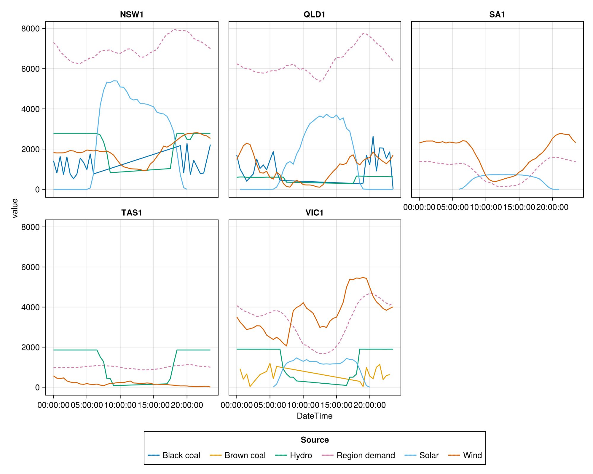

Let's observe the dispatch of a few thermal generators

function filter_non_all_zero(df, group_by, value)
    gdf = groupby(df, group_by)
    is_all_zero = combine(gdf, :value => (x -> all(x == 0)) => :all_zero)
    subset!(is_all_zero, :all_zero => x -> .!x)
    return innerjoin(df, is_all_zero, on = group_by)
end

begin
    thermals_non_zero = filter_non_all_zero(thermal, :name, :value)
    sample = first(unique(thermals_non_zero.name), 5)
    sample = subset!(thermals_non_zero, :name => ByRow(in(sample)))
    data(sample) * mapping(:DateTime, :value, color = :name) * visual(Lines) |> draw
end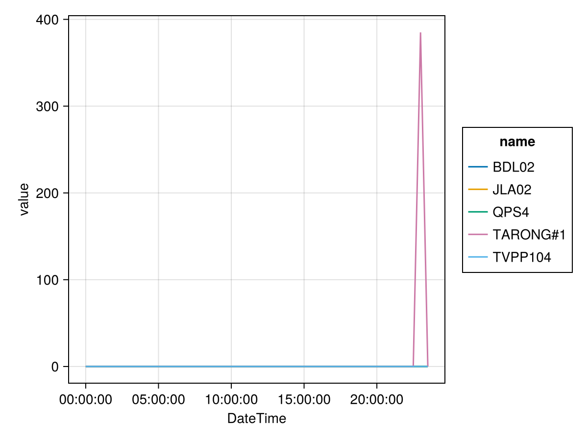

Let's observe the dispatch of a few renewable generators

begin
    renewables_non_zero = filter_non_all_zero(renewables, :name, :value)
    sample = first(unique(renewables_non_zero.name), 5)
    sample = subset!(renewables_non_zero, :name => ByRow(in(sample)))
    data(sample) * mapping(:DateTime, :value, color = :name) * visual(Lines) |> draw
end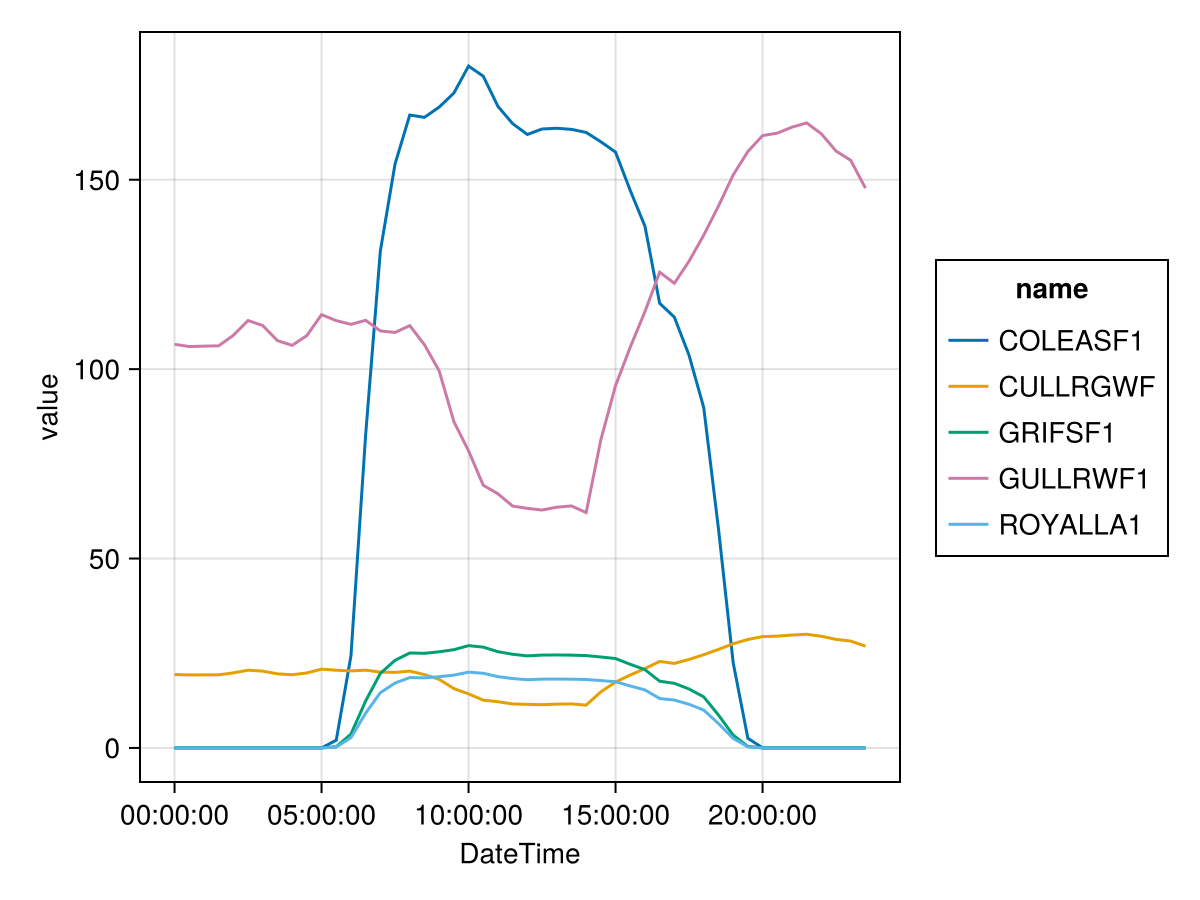

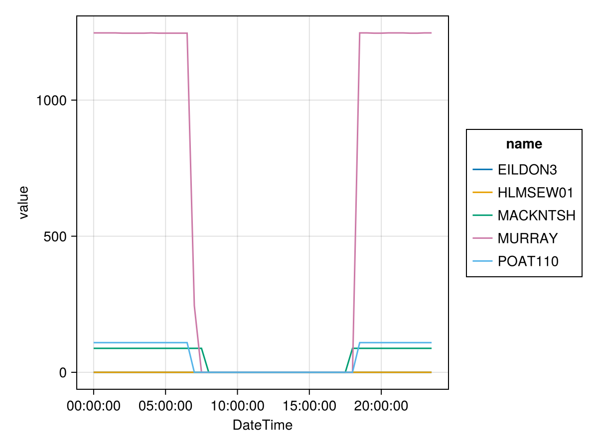
Let's observe the dispatch of a few hydro generators

begin
    hydro_non_zero = filter_non_all_zero(hydro, :name, :value)
    sample = first(unique(hydro_non_zero.name), 5)
    sample = subset!(hydro_non_zero, :name => ByRow(in(sample)))
    data(sample) * mapping(:DateTime, :value, color = :name) * visual(Lines) |> draw
end